Variable Shipping Costs
 PREVIOUS
NEXT
| > Discrete Optimization > Transport: Piecewise Linear Optimization > Describing the Problem > Variable Shipping Costs |
Variable Shipping Costs |
INDEX
 PREVIOUS
NEXT
|
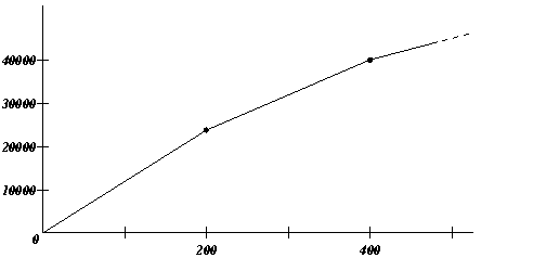
Now consider the costs of shipping from a given factory to a given showroom. Assume that for every pair (factory, showroom), there are different rates, varying according to the quantity shipped. To illustrate the difference between convex and concave piecewise linear functions, in fact, this example assumes that there are two different tables of rates for shipping cars from factories to showrooms. The first table of rates looks like this:
These costs that vary according to quantity define the piecewise linear function represented in Figure 16.3. As you see, the slopes of the segments of that function are decreasing, so that function is concave.

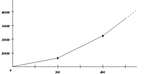
Also assume that there is a second table of rates for shipping cars from factories to showrooms. The second table of rates looks like this:
The costs in this second table of rates that vary according to the quantity of cars shipped define a piecewise linear function, too. It appears in Figure 16.4. The slopes of the segments in this second piecewise linear function are increasing, so this function is convex.

| Copyright © 1987-2003 ILOG, S.A. All rights reserved. Legal terms. | PREVIOUS NEXT |