Discontinuous Piecewise Linear Functions

INDEX PREVIOUS NEXT

Thus far, you have seen a piecewise linear function where the segments are continuous. Intuitively, in a continuous piecewise linear function, the endpoint of one segment has the same coordinates as the initial point of the next segment, as in Figure 16.1.

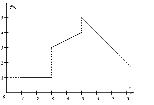
There are piecewise linear functions, however, where two consecutive breakpoints may have the same x coordinate but differ in the value of f(x). Such a difference is known as a step in the piecewise linear function, and such a function is known as discontinuous. Figure 16.2 shows a discontinuous piecewise linear function with two steps.

• The value of the first point of a step in the array of slopes is the height of the step.
• The value of the second point of the step in the array of slopes is the slope of the function after the step.

By convention, a breakpoint belongs to the segment that starts at that breakpoint. For example, in Figure 16.2, f(3) is equal to 3 (not 1); similarly, f(5) is equal to 5.

In Concert Technology, a discontinuous piecewise linear function is represented as an instance of the class IloPiecewiseLinear (the same class as used for continuous piecewise linear functions). For example, the function in Figure 16.2 is declared in this way:

IloPiecewiseLinear(x, 
                   IloNumArray(env, 4, 3. ,3. ,5. ,5.),
                   IloNumArray(env, 5, 0., 2., 0.5, 1., -1.),
                   0, 1);